To use this notebook we will be using a branch of mtpy-v2 that is not released yet. We will also be using panel applications for more interactive plotting.

To create an environment in conda:

conda create -n mt python=3.14
pip install mtpy-v2
pip install jupyterlab

To install the beta version of mtpy-v2

pip install git+https://github.com/MTgeophysics/mtpy-v2.git@bokeh
pip install bokeh jupyter_bokeh

Load in data¶

Here we will load in a transfer functions from all of SAGE around the Valles Caldera as edi files and save them to a HDF5 file.

from pathlib import Path
from mtpy import MTData, MTCollection

import panel as pn
pn.extension(comms='vscode')

h5_exists = True
if h5_exists is False:  
    edi_path = Path(r"c:\Users\jpeacock\OneDrive - DOI\SAGE\EDI_Files\renamed")
    md = MTData()
    md.add_station(list(edi_path.glob("*.edi")))
    with MTCollection() as mc:
        mc.open_collection(r"c:\Users\jpeacock\OneDrive - DOI\SAGE\sage_2026.h5")
        mc.from_mt_data(md)
    h5_exists = True
elif h5_exists is True:
    with MTCollection() as mc:
        mc.open_collection(r"c:\Users\jpeacock\OneDrive - DOI\SAGE\sage_2026.h5")
        md = mc.to_mt_data()

26:06:27T07:09:21 | INFO | line:1035 |mth5.mth5 | close_mth5 | Flushing and closing c:\Users\jpeacock\OneDrive - DOI\SAGE\sage_2026.h5

Plot Station Locations¶

This will plot stations on a basemap. You can change a few parameters like station symbol and color and the basemap.

station_plot = md.plot_stations()
station_plot.panel().servable()

Plot MT Response¶

Here we will plot the MT response for a single station, but you can plot multiple stations in one.

plot_mt_responses = md.plot_mt_responses()
plot_mt_responses.panel().servable()

Plot Phase Tensor Maps¶

plot_pt_map = md.plot_phase_tensor_map()
plot_pt_map.panel().servable()

Plot Geoelectric Strike¶

plot_strike = md.plot_strike()
plot_strike.panel().servable()

Extract a Profile¶

md.utm_epsg = 32613

profile = md.get_profile(-106.5, 35.96, -106.3, 35.96, 1500)

plot profile stations¶

profile_stations = profile.plot_stations()
profile_stations.panel().servable()

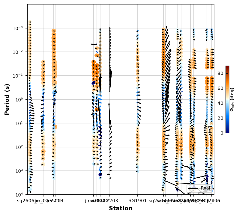
Plot Profile Pseudosections¶

profile_pt_ps = profile.plot_phase_tensor_pseudosection(backend="matplotlib")
profile_pt_ps.x_stretch = 5
profile_pt_ps.plot_tipper = "yr"
profile_pt_ps.plot()

profile_res_ps = profile.plot_resistivity_phase_pseudosections()
profile_res_ps.panel().servable()

1D inversion¶

from mtpy.imaging.bokeh_plots.panel_simpeg1d_app import Simpeg1DPanelApp

simpeg_app = Simpeg1DPanelApp(md)

---------------------------------------------------------------------------
TypeError                                 Traceback (most recent call last)
Cell In[10], line 4
      1 from mtpy.imaging.bokeh_plots.panel_simpeg1d_app import Simpeg1DPanelApp
      2 
      3 simpeg_app = Simpeg1DPanelApp(md)
----> 4 simpeg_app.view()

TypeError: 'Column' object is not callable